So you are working on text identification or face detection, and the question that arises is which algorithm to use and what will be the performance.
I am doing a project where I need to use SVM for detecting cyber attacks, but in order to identify them, I need to learn what makes this algorithm so good. For this project, I will be learning the basics of SVM with real-world examples, and once we are done with the examples, we will try the real project.
What is SVM?
Before we begin, we should understand what SVM is. In my opinion, SVM is a machine learning model that can be used for classification or regression problems.
What exactly is classfication and regression? In simpliest term Regression alogrothium is when there is a relatin between two variable, for example the price house and the size of the house. Classfication alogrothium are those alogo that will find a function and then using that function dvide the data set into two main parts, then alog will train on that sub data set and will identify the 0 value or 1 value.
A support vector machine (SVM) is a supervised machine learning model that uses classification algorithms for two-group classification problems. After giving an SVM model sets of labeled training data for each category, they’re able to categorize new text.
How does SVM Work?
SVM can work in a variety of ways and on a variety of data types; the data can be linear (in one line) or non-linear (data is spread throughout a graph).
The operation is straightforward, but there are ways to use SVM to optimise and get the most out of the SVM Machine Learning Model.
Working with Linear Data:
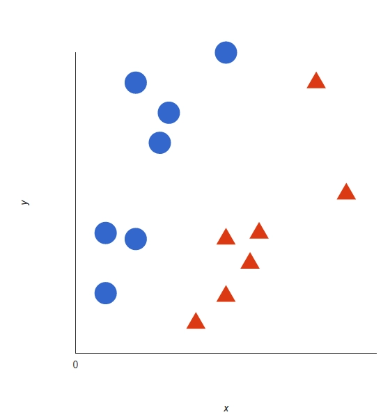
The basics of the support vector machine and how it will work can be easily explained with an example. Consider a data set that contains two features, x and y, each represented by a different colour (red or blue) and each with its own shape (circle or triangle, respectively). Now we will plot the dataset, and we will get this graph.
A Support Vector Machine tasks those data points and then uses a function called hyperplane to create a best sperate boundary with tags. This line is the decision boundary. Everything on the right side is considered blue, and everything on the left side is considered red.
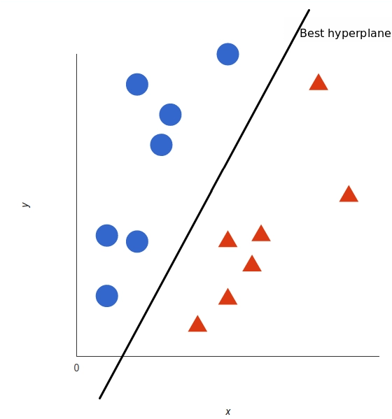
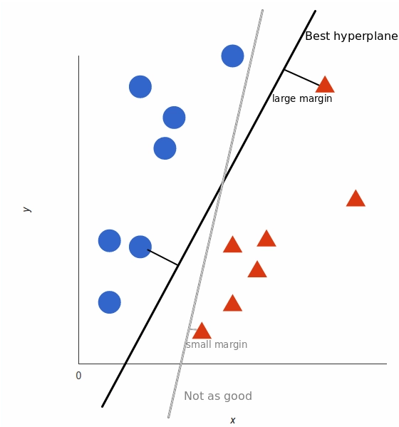
But, what exactly is the best hyperplane? For SVM, it’s the one that maximizes the margins from both tags. In other words: the hyperplane (remember it’s a line in this case) whose distance to the nearest element of each tag is the largest.
Working with Non-Linear Data:
The above example is very simple, and in the real world, data will not be much more linear; it is always going to spread in multiple directions, and there can be more than two variables. So what will you do when there are more than two interacting variables?
Let’s understand this with an example, and your use case might look like this:
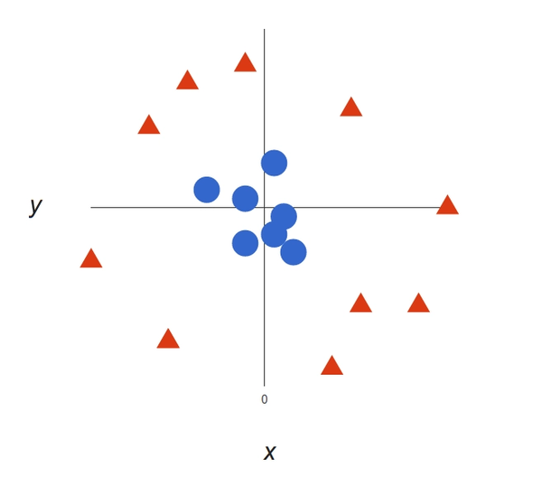
It’s pretty clear that there’s not a linear decision boundary (a single straight line that separates both tags). However, the vectors are very clearly segregated and it looks as though it should be easy to separate them.
So to solve it, we will be adding a third dimension. Uptill now we have only two dimension x and y but Now we will be creating Z as a third dimension, and we rule that it be calculated a certain way that is convenient for us: z = x² + y² (you’ll notice that’s the equation for a circle).
This will give us a three-dimensional space. Taking a slice of that space, it looks like this: !(image-05)[/images/2023/Machine-Learning/SVM/image-05.png]
Now you can see there are two groups, and Now we can use SVM and use a hyperplan.
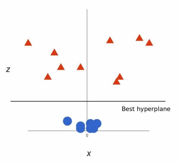
That’s great! Note that since we are in three dimensions now, the hyperplane is a plane parallel to the x axis at a certain z (let’s say z = 1).
What’s left is mapping it back to two dimensions:
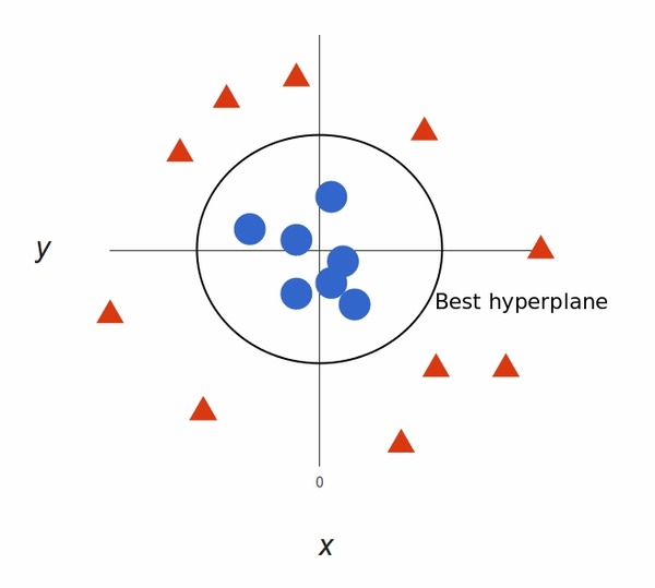
In above plot, points to consider are:
- All values for z would be positive always because z is the squared sum of both x and y
- In the original plot, red circles appear close to the origin of x and y axes, leading to lower value of z and star relatively away from the origin result to higher value of z.
In the SVM classifier, it is easy to have a linear hyper-plane between these two classes. But, another burning question which arises is, should we need to add this feature manually to have a hyper-plane. No, the SVM algorithm has a technique called the kernel trick. The SVM kernel is a function that takes low dimensional input space and transforms it to a higher dimensional space i.e. it converts not separable problem to separable problem. It is mostly useful in non-linear separation problem. Simply put, it does some extremely complex data transformations, then finds out the process to separate the data based on the labels or outputs you’ve defined.
Fine Tune SVM Model:
Tuning Parameters
As we saw in the previous section choosing the right kernel is crucial, because if the transformation is incorrect, then the model can have very poor results. As a rule of thumb, always check if you have linear data and in that case always use linear SVM (linear kernel). Linear SVM is a parametric model, but an RBF kernel SVM isn’t, so the complexity of the latter grows with the size of the training set. Not only is more expensive to train an RBF kernel SVM, but you also have to keep the kernel matrix around, and the projection into this “infinite” higher dimensional space where the data becomes linearly separable is more expensive as well during prediction. Furthermore, you have more hyperparameters to tune, so model selection is more expensive as well! And finally, it’s much easier to overfit a complex model!
Regularization
The Regularization Parameter (in python it’s called C) tells the SVM optimization how much you want to avoid miss classifying each training example.
If the C is higher, the optimization will choose smaller margin hyperplane, so training data miss classification rate will be lower.
On the other hand, if the C is low, then the margin will be big, even if there will be miss classified training data
Gamma
The next important parameter is Gamma. The gamma parameter defines how far the influence of a single training example reaches. This means that high Gamma will consider only points close to the plausible hyperplane and low Gamma will consider points at greater distance.
Decreasing the Gamma will result that finding the correct hyperplane will consider points at greater distances so more and more points will be used (green lines indicates which points were considered when finding the optimal hyperplane).
Margin
The last parameter is the margin. We’ve already talked about margin, higher margin results better model, so better classification (or prediction). The margin should be always maximized.
How to implementation SVM model in Python:
Simple Linear Data set:
- Import Python Libraries:
import numpy as np
import matplotlib.pyplot as plt
from sklearn import svm, datasets
- Import Data Set:
iris = datasets.load_iris()
X = iris.data[:, :2] # we only take the first two features. We could
 # avoid this ugly slicing by using a two-dim dataset
y = iris.target
- Loading SVM Model
# SVM regularization parameter
C = 1.0
# When gama is not initialized then the value will be default value which is 0  but don't define 0 value because it will through an error
svc = svm.SVC(kernel='linear', C=1).fit(X, y)
- Create a mesh to plot
x_min, x_max = X[:, 0].min() - 1, X[:, 0].max() + 1
y_min, y_max = X[:, 1].min() - 1, X[:, 1].max() + 1
h = (x_max / x_min)/100
xx, yy = np.meshgrid(np.arange(x_min, x_max, h),np.arange(y_min, y_max, h))
plt.subplot(1, 1, 1)
Z = svc.predict(np.c_[xx.ravel(), yy.ravel()])
Z = Z.reshape(xx.shape)
plt.contourf(xx, yy, Z, cmap=plt.cm.Paired, alpha=0.8)
plt.scatter(X[:, 0], X[:, 1], c=y, cmap=plt.cm.Paired)
plt.xlabel('Sepal length')
plt.ylabel('Sepal width')
plt.xlim(xx.min(), xx.max())
plt.title('SVC with linear kernel')
plt.show()
Pros and Cons associated with SVM
- Pros:
- It works really well with a clear margin of separation
- It is effective in high dimensional spaces.
- It is effective in cases where the number of dimensions is greater than the number of samples.
- It uses a subset of training points in the decision function (called support vectors), so it is also memory efficient.
- Cons:
- It doesn’t perform well when we have large data set because the required training time is higher
- It also doesn’t perform very well, when the data set has more noise i.e. target classes are overlapping
- SVM doesn’t directly provide probability estimates, these are calculated using an expensive five-fold cross-validation. It is included in the related SVC method of Python scikit-learn library.
Reference
Here are some of the references and research papers that I used to understand the support vector machine model. If you are facing any problems, here are some links.
Articles References:
Video References:
Credit:
This article was written by Abdul Rafay and published on Future Insight.
Contact Us:
If you have any questions, please contact
Future Insight:
Author:
Abdul Rafay:
I will see you next time❤️.
Thumbnail: